Syntactic Processing
Syntactic processing is widely used in applications such as question answering systems, information extraction, sentiment analysis, grammar checking etc. There are 3 broad levels of syntactic processing:
(Parts-of-Speech) POS tagging
Constituency parsing
Dependency parsing
POS tagging is a crucial task in syntactic processing and is used as a preprocessing step in many NLP applications
POS tagging
The four main techniques used for POS tagging:
Lexicon-based approach uses the following simple statistical algorithm: for each word, it assigns the POS tag that most frequently occurs for that word in some training corpus. For example, it will assign the tag “verb” to any occurrence of the word “run” if “run” is used as a verb more often than any other tag.
Rule-based taggers first assign the tag using the lexicon method and then apply predefined rules. Some examples of rules are: Change the tag to VBG for words ending with ‘-ing’, Changes the tag to VBD for words ending with ‘-ed’, etc.
Probabilistic (or stochastic) techniques don’t naively assign the highest frequency tag to each word, instead, they look at slightly longer parts of the sequence and often use the tag(s) and the word(s) appearing before the target word to be tagged. The commonly used probabilistic algorithm for POS tagging is Hidden Markov Model (HMM)
Deep-learning based POS tagging: Recurrent Neural Networks (RNNs) are used for sequential modeling processes
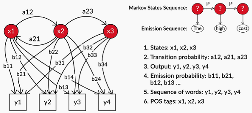
Hidden Markov Models
Markov processes are commonly used to model sequential data, such as text and speech. The first-order Markov assumption states that the probability of an event (or state) depends only on the previous state. The Hidden Markov Model, an extension to the Markov process, is used to model phenomena where the states are hidden and they emit observations. The transition and the emission probabilities specify the probabilities of transition between states and emission of observations from states, respectively. In POS tagging, the states are the POS tags while the words are the observations. To summarise, a Hidden Markov Model is defined by the initial state, emission, and the transition probabilities.
The POS tag for given word depends on two things: POS tag of the previous word and the word itself.
So, the probability of a tag sequence … for a given the word sequence … can be defined as:
For a sequence of words and tags, a total of tag sequences are possible.
Viterbi Heuristic
Viterbi Heuristic can deal with this problem by taking a greedy approach. The basic idea of the Viterbi algorithm is as follows - given a list of observations (words) to be tagged, rather than computing the probabilities of all possible tag sequences, you assign tags sequentially, i.e. assign the most likely tag to each word using the previous tag.
More formally, you assign the tag to each word such that it maximises the likelihood:
where is the tag assigned to the previous word. The probability of a tag is assumed to be dependent only on the previous tag , and hence the term - Markov Assumption.
Viterbi algorithm is an example of a dynamic programming algorithm. In general, algorithms which break down a complex problem into subproblems and solve each subproblem optimally are called dynamic programming algorithms.
Learning HMM Model Parameters
The process of learning the probabilities from a tagged corpus is called training an HMM model. The emission and the transition probabilities can be learnt as follows:
Emission Probability of a word for tag : = Number of times has been tagged /Number of times appears
Example: = Number of times ‘dog’ appears as Noun/ Number of times Noun is appearing
Transition Probability of tag followed by tag : = Number of times is followed by tag / Number of times appears
Example: = number of times adjective is followed by Noun/ Number of times Adjective is appearing
Constituency Parsing
shallow parsing is not sufficient. Shallow parsing, as the name suggests, refers to fairly shallow levels of parsing such as POS tagging, chunking, etc. But such techniques would not be able to check the grammatical structure of the sentence, i.e. whether a sentence is grammatically correct, or understand the dependencies between words in a sentence.
Two most commonly used paradigms of parsing - constituency parsing and dependency parsing, which would help to check the grammatical structure of the sentence.
In constituency parsing, you learnt the basic idea of constituents as grammatically meaningful groups of words, or phrases, such as noun phrase, verb phrase etc. You also learnt the idea of context-free grammars or CFGs which specify a set of production rules. Any production rule can be written as A -> B C, where A is a non-terminal symbol (NP, VP, N etc.) and B and C are either non-terminals or terminal symbols (i.e. words in vocabulary such as flight, man etc.).
Example a CFG is:
S -> NP VP
NP -> DT N| N| N PP
VP -> V| V NP
N -> ‘woman’| ‘bear’
V -> ‘ate’
DT -> ‘the’| ‘a’
There are two broad approaches to constituency parsing:
Top-down parsing: starts with the start symbol at the top and uses the production rules to parse each word one by one. And, you continue to parse until all the words have been allocated to some production rule.
Top-down parsers have a specific limitation- Left Recursion.
Example of a left recursion: VP -> VP NP. Whenever a top-down parser encounters such a rule, it runs into an infinite loop, thus no parse tree is obtained. Following is the illustration of top-down parse:
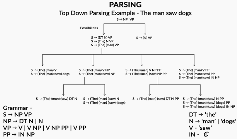
Figure 2:Top-down parse
Bottom-up parsing: reduces each terminal word to a production rule, i.e. reduces the right-hand-side of the grammar to the left-hand-side. It continues the reduction process until the entire sentence has been reduced to the start symbol S. Shift-Reduce Parser algorithm, which parses the words of the sentence one-by-one either by shifting a word to the stack or reducing the stack by using the production rules. Below is an example of bottom-up parse tree.
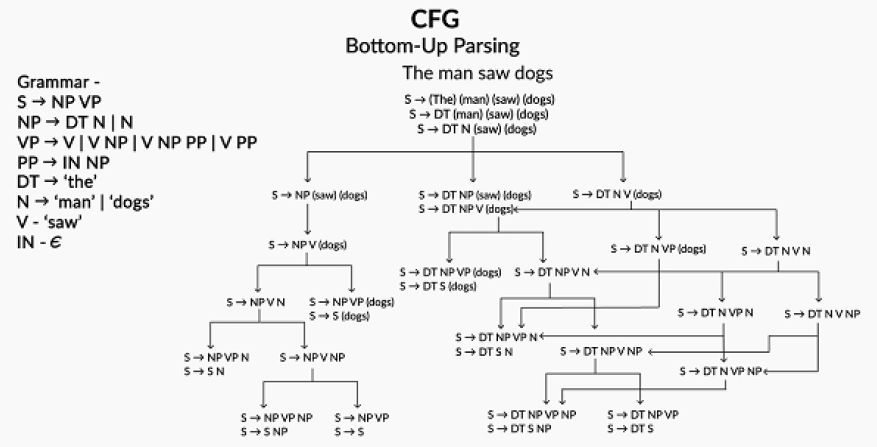
Figure 3:Bottom-up parse
Probabilistic CFG
Since natural languages are inherently ambiguous, there are often cases where multiple parse trees are possible. In such cases, we need a way to make the algorithms figure out the most likely parse tree. Probabilistic Context-Free Grammars (PCFGs) are used when we want to find the most probable parsed structure of the sentence. PCFGs are grammar rules, similar to what you have seen before, along with probabilities associated with each production rule. An example production rule is as follows:
NP -> Det N (0.5) | N (0.3) |N PP (0.2)
It means that the probability of an NP breaking down to a ‘Det N’ is 0.50, to an ‘N’ is 0.30 and to an ‘N PP’ is 0.20. Note that the sum of probabilities is 1.00. Overall probability for a parsed structure of the sentence is probabilities of all rules used in that parsed structure. The parsed tree with maximum probability is best possible interpretation of the sentence.
Chomsky Normal Form
The Chomsky Normal Form (CNF), proposed by the linguist Noam Chomsky, is a normalized version of the CFG with a standard set of rules defining how production rule must be written. The three forms of CNF rules can be written:
A -> B C
A -> a
S -> ε
A, B, C are non-terminals (POS tags), a is a terminal (term), S is the start symbol of the grammar and ε is the null string. The table below shows some examples for converting CFGs to the CNF:
| CFG | VP -> V NP PP | VP -> V | | CNF | VP -> V (NP1) | VP -> V (VP1) | | | NP1 -> NP PP | VP1 -> ε |
Dependency Parsing
In dependency grammar, constituencies (such as NP, VP etc.) do not form the basic elements of grammar, but rather dependencies are established between the words themselves.
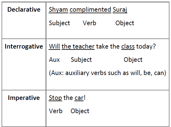
Free word order languages such as Hindi, Bengali are difficult to parse using constituency parsing techniques. This is because, in such free-word-order languages, the order of words/constituents may change significantly while keeping the meaning exactly the same. It is thus difficult to fit the sentences into the finite set of production rules that CFGs offer. Dependencies in a sentence are defined using the elements Subject-Verb-Object (SVO). The following table shows SVO dependencies in three types of sentences - declarative, interrogative, and imperative
Apart from dependencies defined in the form of subject-verb-object, there’s a non-exhaustive list of dependency relationships, which are called universal dependencies.
Dependencies are represented as labelled arcs of the form where ‘’ is called the “head” of the dependency, ‘’ is the “dependent” and is the “label” assigned to the arc. In a dependency parse, we start from the root of the sentence, which is often a verb. And then start to establish dependencies between root and other words.
Information Extraction
Information Extraction (IE) system can extract entities relevant for booking flights (such as source and destination cities, time, date, budget constraints etc.) in a structured format from unstructured user-generated input. IE is used in many applications such as chatbots, extracting information from websites, etc.
A generic pipeline for Information Extraction is as follows:
Preprocessing:
Sentence Tokenization: sequence segmentation of text
Word Tokenization: breaks down sentences into tokens
POS tagging: assigning Parts of Speech tags to the tokens. The POS tags can be helpful in defining what words could form an entity
Entity Recognition:
Rule-based models
Probabilistic models
Most IE pipelines start with the usual text preprocessing steps - sentence segmentation, word tokenisation and POS tagging. After preprocessing, the common tasks are Named Entity Recognition (NER), and optionally relation recognition and record linkage. NER is arguably the most important and non-trivial task in the pipeline. There are various techniques and models for building Named Entity Recognition (NER) system, which is a key component in information extraction systems:
Rule-based techniques
Regular expression based techniques
Chunking
Probabilistic models
Unigram & Bigram models
Naive Bayes Classifier
Decision trees
Conditional Random Fields (CRFs)
IOB (or BIO) method tags each token in the sentence with one of the three labels: I - inside (the entity), O- outside (the entity) and B - beginning (of entity). You saw that IOB labeling is especially helpful if the entities contain multiple words. For example: words like ‘Delta Airlines’, ‘New York, etc, are single entities.
Rule-based method for NER
Chunking is a common shallow parsing technique used to chunk words that constitute some meaningful phrase in the sentence. A noun phrase chunk (NP chunk) is commonly used in NER tasks to identify groups of words that correspond to some ‘entity’.
Sentence: She bought a new car from the BMW showroom.
Noun phrase chunks: a new car, the BMW showroom
The idea of chunking in the context of entity recognition is simple - most entities are nouns and noun phrases, so rules can be written to extract these noun phrases and hopefully extract a large number of named entities. Example of chunking done using regular expressions:
Sentence: John booked the hotel.
Noun phrase chunks: ‘John’, ‘the hotel’
Grammar:
Probabilistic method for NER
The following two probabilistic models to get the most probable IOB tags for word:
Unigram chunker computes the unigram probabilities P(IOB label | pos) for each word and assigns the label that is most likely for the POS tag.
Bigram chunker works similar to a unigram chunker, the only difference being that now the probability of a POS tag having an IOB label is computed using the current and the previous POS tags, i.e. P(label | pos, prev_pos).
Gazetteer Lookup, another way to identify named entities (like cities and states) is to look up a dictionary or a gazetteer. A gazetteer is a geographical directory which stores data regarding the names of geographical entities (cities, states, countries) and some other features related to the geographies.
Naive Bayes and Decision Tree classifier can also be used in NER.
Conditional Random Fields
HMMs can be used for any sequence classification task, such as NER. However, many NER tasks and datasets are far more complex than tasks such as POS tagging, and therefore, more sophisticated sequence models have been developed and widely accepted in the NLP community. One of these models is Conditional Random Fields (CRFs).
CRFs are used in a wide variety of sequence labelling tasks across various domains - POS tagging, speech recognition, NER, and even in computational biology for modelling genetic patterns etc. CRFs model the conditional probability , where is the vector of output sequence (IOB labels here) and is the input sequence (words to be tagged), which are similar to Logistic Regression classifier. Broadly, there are two types of classifiers in ML:
Discriminative classifiers learn the boundary between classes by modelling the conditional probability distribution , where is the vector of class labels and represents the input features. Examples are Logistic Regression, SVMs etc.
Generative classifiers model the joint probability distribution . Examples of generative classifiers are Naive Bayes, HMMs etc.
CRFs use ‘feature functions’ rather than the input word sequence itself. The idea is similar to how features are extracted for building the naive Bayes and decision tree classifiers in a previous section. Some example ‘word-features’ (each word has these features) are:
Word and POS tag based features: word_is_city, word_is_digit, pos, previous_pos, etc.
Label-based features: previous_label
A feature function takes the following four inputs:
The input sequence of words:
The position of a word in the sentence (whose features are to be extracted)
The label of the current word (the target label)
The label of the previous word
Let’s see an example of a feature function:
A feature function which returns 1 if the word is a city and the corresponding label is ‘I-location’, else 0. This can be represented as:
The feature function returns 1 only if both the conditions are satisfied, i.e. when the word is a city name and is tagged as ‘I-location’ (e.g. Tokyo/I-location).
Every feature function has a weight associated with it, which represents the ‘importance’ of that feature function. This is almost exactly the same as logistic regression where coefficients of features represent their importance. Training a CRF means to compute the optimal weight vector which best represents the observed sequences for the given word sequences . In other words, we want to find the set of weights which maximises .
In CRFs, the conditional probabilities are modeled using a scoring function. If there are feature functions (and thus weights), for each word in the sequence , a scoring function for a word is defined as follows:
and the overall sequence score for the sentence can be defined as:
The probability of observing the label sequence given the input sequence is given by:
where is sum of scores of all possible tag sequences
Training a CRF model means to compute the optimal set of weights which best represents the observed sequences for the given word sequences . In other words, we want to find the set of weights which maximises the conditional probability for all the observed sequences , by taking log and simplifying the equations and adding a regularization term to prevent overfitting, the final equation comes out as:
The inference task to assign the label sequence to which maximises the score of the sequence, i.e.
The naive way to get is by calculating for every possible label sequence , and then choose the label sequence that has maximum value. However, there are an exponential number of possible labels ( for a tag set of size and a sentence of length ), and this task is computationally heavy.