Neural Network¶

Perceptrons were one of the earliest proposed models for learning simple classification tasks, which later became the fundamental building block of artificial neural networks.

Artificial Neuron¶

An artificial neuron is very similar to a perceptron, except that the activation function is not a step function.

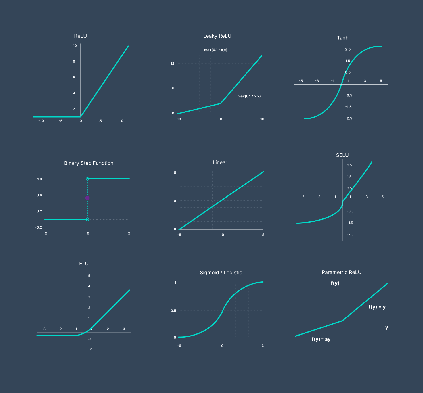
Like a perceptron, the input is the weighted sum of inputs. The output is the activation function applied on the input. The activation function could be any function, though it should have some important properties such as:

Activation functions should be smooth i.e. they should have no abrupt changes when plotted
They should also make the inputs and outputs non-linear with respect to each other to some extent. This is because non-linearity helps in making neural networks more compact

Some of the common activation functions are as follows:

An artificial neural network is a network of such neurons. Neurons in a neural network are arranged in layers. The first and the last layer are called the input and output layers. Input layers have as many neurons as the number of attributes in the data set and the output layer has as many neurons as the number of classes of the target variable (for a classification problem). For a regression problem, the number of neurons in the output layer would be 1 (a numeric variable). There are six main things that need to be specified for specifying a neural network completely:

Network Topology
Input Layer
Output Layer
Weights
Activation functions
Biases

An important thing to note is that the inputs can only be numeric. For different types of input data, we use different ways to convert the inputs to a numeric form. In case of text data, we either use a one-hot vector or word embeddings corresponding to a certain word. Feeding images (or videos) is straightforward since images are naturally represented as arrays of numbers.

The output layer used in case of multiclass classification problem is the softmax layer. A softmax output is a multiclass logistic function commonly used to compute the ‘probability’ of an input belonging to one of the multiple classes.

Since large neural networks can potentially have extremely complex structures, certain assumptions are made to simplify the way information flows in them:

Neurons are arranged in layers and the layers are arranged sequentially
Neurons within the same layer do not interact with each other
All the inputs enter the network through the input layer and all the outputs go out of the network through the output layer
Neurons in consecutive layers are densely connected, i.e. all neurons in layer $l$ are connected to all neurons in layer $l+1$
Every interconnection in the neural network has a weight associated with it, and every neuron has a bias associated with it
All neurons in a particular layer use the same activation function

Neural networks require rigorous training. Recall that models such as linear regression, logistic regression, SVMs etc. are trained on their coefficients, i.e. the training task is to find the optimal values of the coefficients to minimize some cost function. Neural networks are no different - they are trained on weights and biases.

During training, the neural network learning algorithm fits various models to the training data and selects the best model for prediction. The learning algorithm is trained with a fixed set of hyperparameters - the network structure (number of layers, number of neurons in the input, hidden and output layers etc.). It is trained on the weights and the biases, which are the parameters of the network.

Neural Networks can be used to reasonably approriximate most functions — Figure 2:Neural Networks can be used to *reasonably* approriximate *most* functions

Feed forward¶

In artificial neural networks, the output from one layer is used as input to the next layer. Such networks are called feedforward neural networks. Feed forward neural network architecture consists of following main parts " Input Layer, Hidden Layer - If the number of hidden layer is one then it is known as a shallow neural network, else it is known as a deep neural network, Output Layer

Backpropagation¶

In the neural network training task the goal is to compute the optimal weights and biases by minimizing some cost function. The task of training neural networks is exactly the same as that of other ML models such as linear regression, SVMs etc. The desired output (output from the last layer) minus the actual output is the cost (or the loss), and we to tune the parameters w and b such that the total cost is minimized.

An important point to note is that if the data is large (which is often the case), loss calculation itself can get pretty messy. For example, if you have a million data points, they will be fed into the network (in batches), the output will be calculated using feedforward and the loss/cost $L_i$ (for $i^{th}$ data point) will be calculated. The total loss is the sum of losses of all the individual data points. We minimize the average of the total loss and the not the total loss. Minimizing the average loss implies that the total loss is getting minimized.

For a large neural network, the number of weight elements and biases becomes so large and minimizing the loss with so many parameters is a difficult task. This complex task is achieved using gradient descent.

For updating weights and biases using plain backpropagation, you have to scan through the entire data set to make a single update to the weights. This is computationally very expensive for large datasets. Thus, you use multiple batches (or mini-batches) of data points, compute the average gradient for a batch, and update the weights based on that gradient.

But there is a danger in doing this - you are making weight updates based only on gradients computed for small batches, not the entire training set. Thus, you make multiple passes through the entire training set using epochs. An epoch is one pass through the entire training set, and you use multiple epochs (typically 10, 20, 50, 100 etc.) while training. In each epoch, you reshuffle all the data points, divide the reshuffled set into m batches, and update weights based on gradient of each batch.

Stochastic Gradient Descent (SGD)¶

In most libraries such as Tensorflow, the SGD training procedure is as follows:

You specify the number of epochs (typical values are 10, 20, 50, 100 etc.) - more epochs require more computational power
You specify the number of batches $m$ (typical values are 32, 64, 128, etc.)
At the start of each epoch, the data set is reshuffled and divided into $m$ batches
The average gradient of each batch is then used to make a weight update
The training is complete at the end of all the epochs

Apart from being computationally faster, the SGD training process has another big advantage - it actually helps you reach the global minima (instead of being stuck at a local minima). Also, to avoid the problem of getting stuck at a local optimum, you need to strike a balance between exploration and exploitation. Exploration means that you try to minimize the loss function with different starting points of $W$ and $b$ , i.e., you initialize $W$ and $b$ with different values. On the other hand, exploitation means that you try to reach the global minima starting from a particular W and b and do not explore the terrain at all. That might lead you to the lowest point locally, but not the necessarily the global minimum.

Modifications in Neural Networks¶

Neural networks are usually large, complex models with tens of thousands of parameters, and thus tend to overfit the training data. As with many other ML models, regularization is a common technique used in neural networks to address this problem.

The ‘parameter norm’ regularization is similar to that in linear regression in almost every aspect. As in lasso regression (L1 norm), we get a sparse weight matrix, which is not the case with the L2 norm. Despite this fact, the L2 norm is more common because the sum of the squares term is easily differentiable which comes in handy during backpropagation. Apart from using the parameter norm, there is another popular neural network regularization technique called dropouts.

Dropouts¶

Some important points to note regarding dropouts are:

Dropouts can be applied only to some layers of the network (in fact, that is a common practice - you choose some layer arbitrarily to apply dropouts to)
The mask $\alpha$ is generated independently for each layer during feedforward, and the same mask is used in backpropagation
The mask changes with each minibatch/iteration, are randomly generated in each iteration (sampled from a Bernoulli with some $p(1)=q$ )

Why the dropout strategy works well is explained through the notion of a manifold. Manifold captures the observation that in high dimensional spaces, the data points often actually lie in a lower-dimensional manifold. The dropout strategy uses this fact to find a lower-dimensional solution to the problem.

Dropouts help in symmetry breaking as well. There is every possibility of the creation of communities within neurons which restricts them from learning independently. Hence, by setting some random set of the weights to zero in every iteration, this community/symmetry is broken. Note that there, a different mini batch is processed in every iteration in an epoch, and dropouts are applied to each mini batch.