Central Limit Theorem¶

Sampling distribution¶

Let’s start with an example, suppose from the SAT math scores

• You take a sample of 10 random students from a population of 100. You might get a mean of 502 for that sample.

• Then, you do it again with a new sample of 10 students. You might get a mean of 480 this time.

• Then, you do it again. And again. And again...... and get the following means for each of those three new samples of 10 people: 550, 517, 472

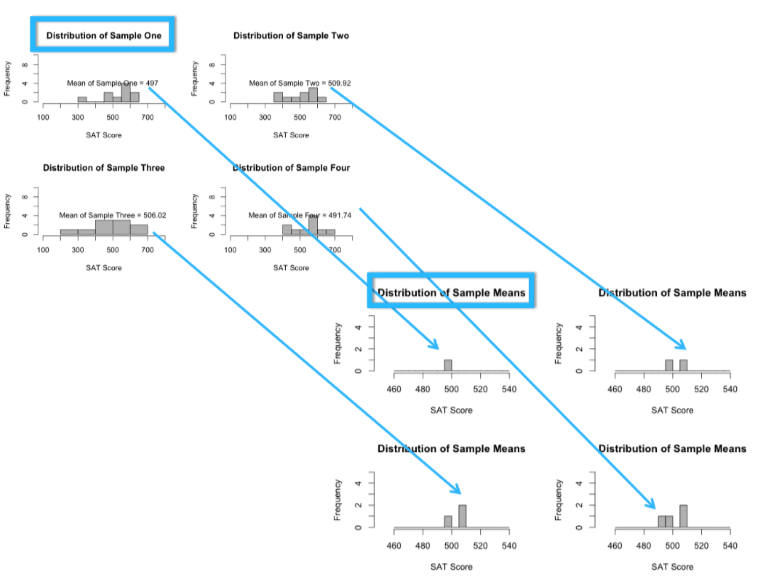
The sampling distribution, which is basically the distribution of sample means of a population, has some interesting properties which are collectively called the central limit theorem, which states that no matter how the original population is distributed, the sampling distribution will follow these three properties -

• Sampling Distribution’s Mean $(\mu_{\bar{x}}) =$ Population Mean $(\mu)$

• Sampling Distribution’s Standard Deviation (Standard Error) $= \sigma\sqrt{n}$, where $\sigma$ is the population’s standard deviation and $n$ is the sample size

• For $n > 30$, the sampling distribution becomes a normal distribution. Strongly skewed distributions can require larger sample sizes.

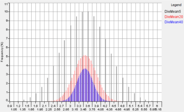
To prove the thrid point let’s take a uniform distribution, in the image below $500,000$ times for each sample size $(5, 20, 40)$ have been drawn and their mean plotted. We’d expect the average to be $(1 + 2 + 3 + 4 + 5 + 6 / 6 = 3.5)$. The sampling distributions of the means center on this value. Just as the central limit theorem predicts, as we increase the sample size, the sampling distributions more closely approximate a normal distribution and have a tighter spread of values.